🛒 How to Run Sales Revenue Analysis and Forecasting With R

I’d probably be the millionth blogger writing it. Still, it’s impossible to deny it: data-driven decision making is essential for every individual or organisation that want to improve efficiency, productivity and returns in life and business.

How? Let’s think about an easy example: A typical bookseller is usually aware of the following facts about its last customers: which books they bought and how much they spent. On the other hand, big-data-driven retailers as Amazon have their online customers produce tons of clued during a single purchase:

• What they were looking for.
• How they navigated through the website.
• Whether and how much they were attracted by promotions, the particular page layout, the reviews, et cetera.

I believe there’s no need to tell you how’s going to win the customer more efficiently.

Guess what? You do not need to be a 1.69 trillion dollars worth of the company to manipulate data and generate meaningful insights to make better decisions. I will try to prove it by analysing the Google Merchandising Store data, transforming them into something “manageable”. After a first analysis of the output, we’ll try to make some forecast. The guiding question here will be: which user source will bring more revenue?

Initialisation

We will use the Google Merchandising Store because it kindly shares all the stats and web analytics by following this guide. In R, will be needing the following libraries.

library(readxl)
library(tidyverse)
library(dplyr)
library(tidyr)
library(fpp)
library(astsa)
library(lubridate)
library(tsutils)
library(smooth)

Collection

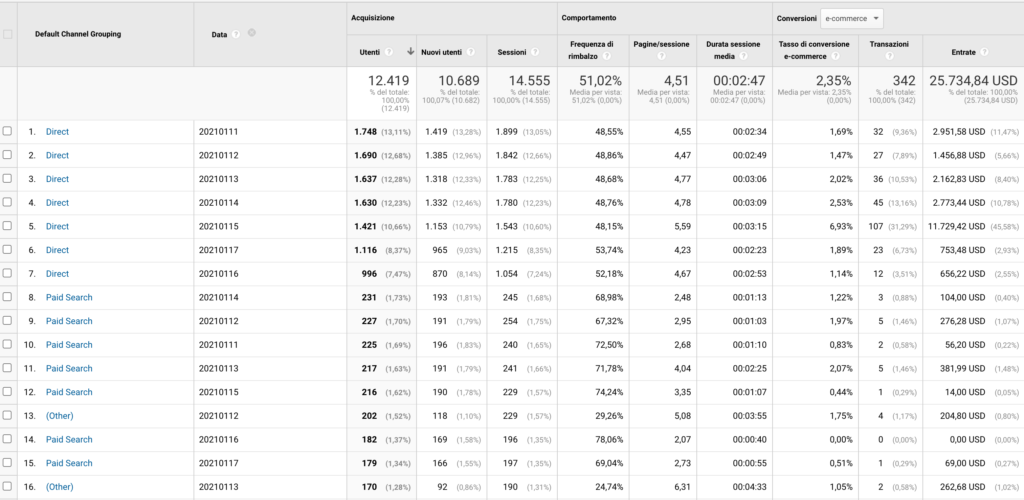
My objective is to have an Excel file reporting the number of users and revenues each source has acquired every day of 2019 and 2020. For example, we would like to know that paid marketing on 20th January of 2019 brought 200 users that made 140 dollars. To do so, let’s go to the acquisition section and create a report with e-commerce goals of 2019 and 2020, where the second dimension was the date. The result should be something like that.

Let’s now exploit R to fix the table. In order to do so, we are going to import the table, format the columns correctly, filter the column and obtain a clean dataset.

# Import the dataset, Factor the channels and convert column date
X2020 <- read_excel("2020.xlsx", sheet = 2)
X2020$`Default Channel Grouping` <-
  as.factor(X2020$`Default Channel Grouping`)
X2020$Data <- as.Date(X2020$Data, format = "%Y%m%d")
X2020$Data <- format(X2020$Data, "%Y-%m")
X2020 <- X2020 %>%
  group_by(`Default Channel Grouping`, Data) %>%
  summarise_if(is.numeric, sum)

# Select few columns and rename them
X2020 <- X2020 %>%
  select(c(`Default Channel Grouping`, Data, Utenti, Entrate, Transazioni))
colnames(X2020) <-
  c("channel", "date", "users", "revenue", "transactions")

# create a first dataframe spreading the row values to the columns values
revenues1 <- X2020 %>%
  select(channel, date, users) %>%
  spread(channel, users, fill = 0)

# create a second dataframe with daily revenues
revenues2 <- X2020 %>%
  group_by(date) %>%
  summarise(sum = sum(revenue))

# create a third dataframe with daily number of transactions
revenues3 <- X2020 %>%
  group_by(date) %>%
  summarise(trans = sum(transactions))

# combine the two dataframe
revenues_final <- inner_join(revenues1, revenues2, "date")
revenues_final <- inner_join(revenues_final, revenues3, "date")

It’s worth noting that we needed to use the spread function to turn columns values into categories. That’s the reason why we broke the data frame in three before generating the final one.

First Analysis

Now our data frame looks way better, and we can start to check the best channels in terms of revenue.

# simple average of revenue
X2020a <- X2020 %>%
  group_by(channel, date) %>%
  summarise(a = mean(users), b = mean(revenue), c = mean(transactions))

Arguably data is already starting to look useful!

Forecast

Another idea to grasp something about what will happen to the Google Merchandising Store would be to apply the Holt Winter method to predict future events. Holt’s two-parameter model, also known as linear, exponential smoothing, is a popular smoothing model for forecasting data trends. Holt’s model has three separate equations that work together to generate a final forecast. The first is a basic smoothing equation that directly adjusts the last smoothed value for the previous period’s trend. The trend itself is updated over time through the second equation, where the trend is expressed as the difference between the last two smoothed values. Finally, the third equation is used to generate the final forecast. Holt’s model uses two parameters, one for the overall smoothing and the other for the trend smoothing equation.

To apply it to all the eight traffic sources, we will write a loop as follows. Notice that we generate a time series of two years divided into 12 months in the middle of the loop.

channels <-
  c(
    "Affiliates",
    "Direct",
    "Display",
    "Organic Search",
    "Paid Search",
    "Referral",
    "Social",
    "(Other)"
  )

# model generation
for (i in 1:8) {
  X2020i <- filter(X2020, channel == channels[i])
  ts <-
    ts(
      X2020i$revenue,
      start = c(2019, 1),
      end = c(2020, 12),
      frequency = 12
    )
  fit1 <- hw(ts, seasonal = "additive", h = 12)
  summary(fit1)
  plot(fit1)
  decomp <- decomp(ts, outplot = 1)
}

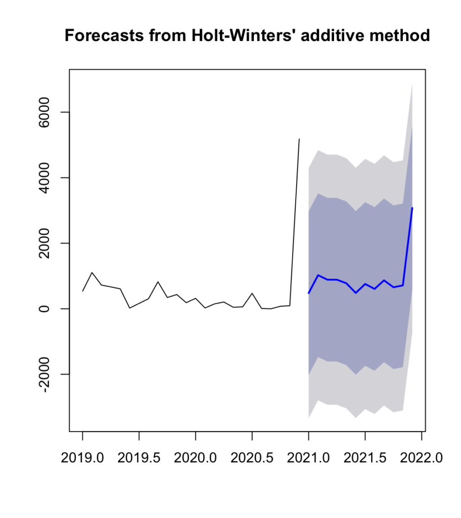
For each of them we will have the following plot, showing us the trend that will follow.

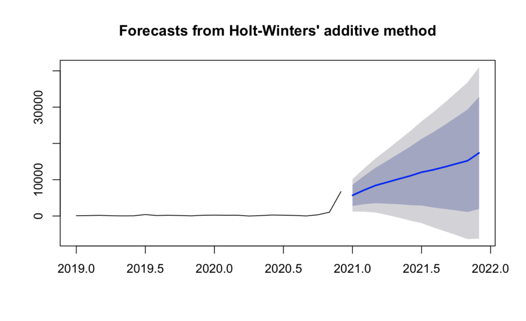
Overall the trend is the following:

Summing up

Based on the forecast and the data already collected, the monthly revenues expected, and the distribution for channel divided for 2021 are the following:

Have you ever tried to forecast some data based on past observations? How was it?